Multidimensional Grid and Data

Introduction

Hi there! The blog posts aim to share how the blocks and threads are organized and how they are used to process multidimensional data. We’ll start with the basics of thread organization and then move our focus to its applications. We’ll demonstrate color-to-gray scale conversion, blurring images and a naive implementation of matrix multiplication in CUDA.

This blog post is written while reading the third chapter, Multidimensional Grids and Data, of the incredible book “Programming Massively Parallel Processors: A Hands-on Approach¹” by Wen-mei W. Hwu, David B. Kirk, and Izzat El Hajj.

Multidimensional Grid Organization

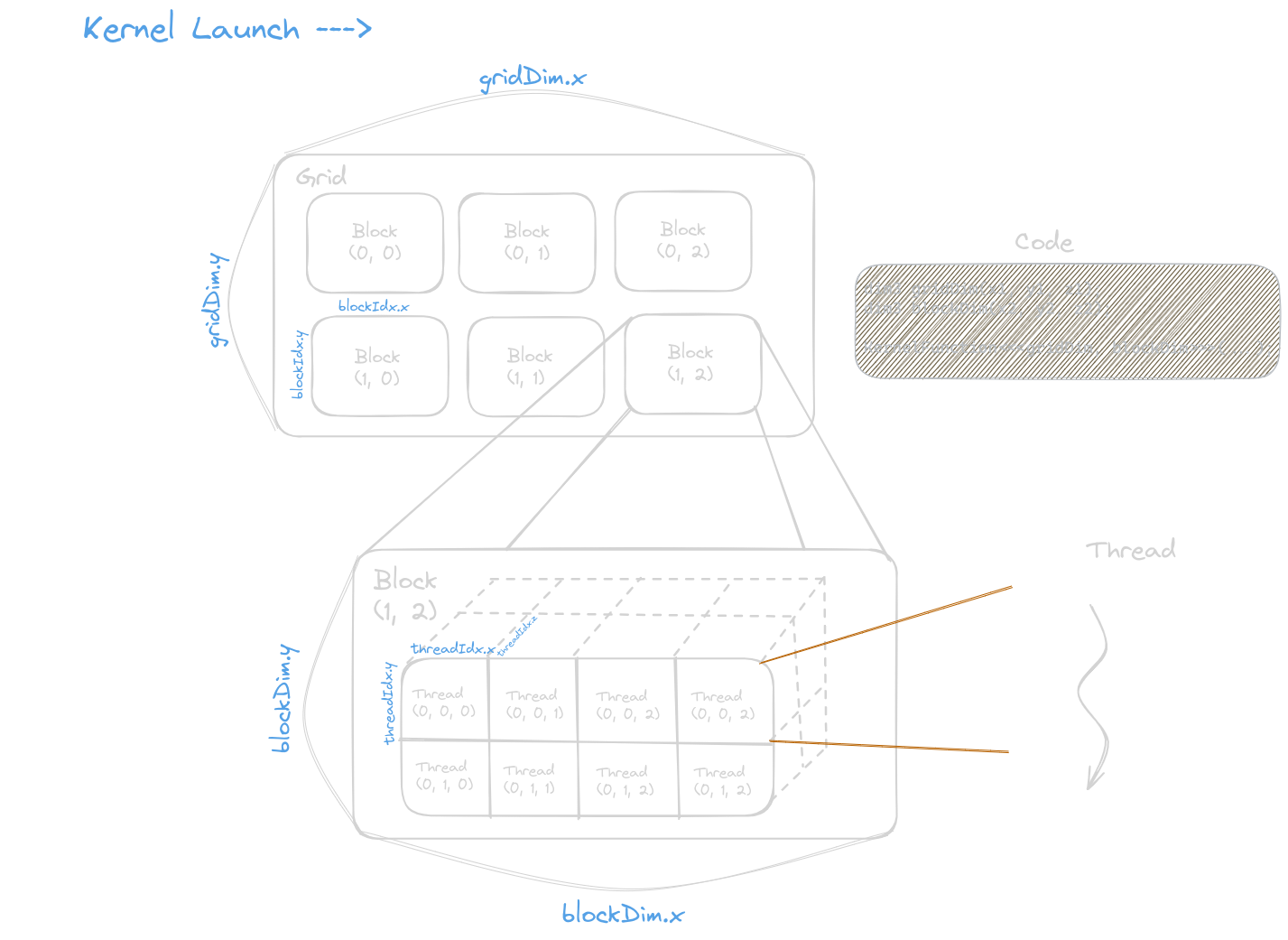
In CUDA, computation is performed in a three-level hierarchy. As soon as the user launches the kernel in device memory, a grid is executed. A grid is a 3D array of blocks. A block is a 3D array of threads. A thread is a simplified view of how a processor executes a sequential program in a modern computer.

Some of the CUDA built-in variables are blockIdx (block index), threadIdx (thread index), gridDim (dimensions of the grid, aka, depicts the number of blocks in a grid), and blockDim (dimensions of the block, aka, depicts the number of threads in a block). To launch a kernel, we need to provide two parameters, as shown below:

// dim3: built-in type of a variable
// dimGrid and dimBlock are host code variables
dim3 dimGrid(32, 1, 1);
dim3 dimBlock(128, 1, 1);

kernelLaunch<<<dimGrid, dimBlock>>>(...);

Notes

• If we want to work on 1D grids and blocks, we can call kernels with integer values instead of declaring them explicitly.
• Allowed values of gridDim.x range from 1 to 2³¹ - 1. And those of gridDim.y and gridDim.z range from 1 to 2⁶ - 1
• The total size of the block in the current CUDA system is limited to 1024 threads.
• All threads in a block have the same blockIdx values, and all blocks in a grid have the same gridIdx values.
• Range of blockIdx.x: 0 to gridDim.x - 1

Color to Gray Scale Conversion

Images are a 2-dimensional array of pixels. To find the co-ordinate of a thread assigned to process the pixel is given by:

Vertical (row co-ordinate) = blockIdx.y * blockDim.y + threadIdx.y;
Horizontal (column co-ordinate) = blockIdx.x * blockDim.x + threadIdx.x;

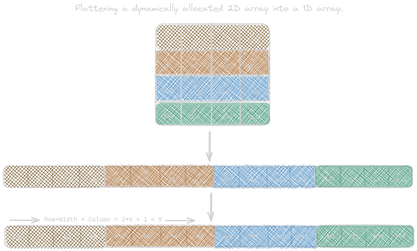
In CUDA C, the information on the number of columns/rows in dynamically allocated arrays is not known at compile time. As a result, programmers need to explicitly linearize, aka flatten, a dynamically allocated 2D or a 3D array into a linear array in the current CUDA C. This is due to the flat memory space in modern computers. We can linearize multidimensional arrays in two different memory format: row-major layout and column-major layout. The figure below shows how to linearize the 2-dimensional array in row-major layout:

Now, let’s write a kernel code for the color to the gray-scale conversion of a 2-dimensional image. It uses the following equation:

L = 0.21*r + 0.72*g + 0.07*b

The CUDA kernel code executed by each thread is given by:

__global__ void colortoGrayscaleConversionKernel(unsigned char* Pout,
                                                 unsigned char* Pin, int width,
                                                 int height) {
    int col = threadIdx.x + blockIdx.x * blockDim.x;
    int row = threadIdx.y + blockIdx.y * blockDim.y;

    // to make sure threads with both row and column are within range
    if (col < width && row < height) {
        // we linearize the memory layout of the data (due to a flat memory
        // space in modern computers)
        // 1D equivalent index for an element of M of row j and column i
        // is j * 4 + i; where 4 is width of matrix (4 x 4)
        int grayOffset = row * width + col;

        // RGB image having CHANNELS times more columns than gray-scale
        int rgbOffset = grayOffset * CHANNELS;
        unsigned char r = Pin[rgbOffset];      // red value
        unsigned char g = Pin[rgbOffset + 1];  // green value
        unsigned char b = Pin[rgbOffset + 2];  // blue value

        // To convert pixel into gray-scale
        Pout[grayOffset] =
            static_cast<unsigned char>(0.21f * r + 0.71f * g + 0.07f * b);
    }
}

Image Blur

Mathematically, an image blurring function calculates the value of an output image pixel as a weighted sum of a patch of pixels encompassing the pixel in the input image. In the code below, we’ll take a simple average value of the N x N patch of pixels of the image. For this kernel, the thread-to-output data mapping remains the same.

__global__ void blurKernel(unsigned char* in, unsigned char* out, int w,
                           int h) {
    int col = threadIdx.x + blockIdx.x * blockDim.x;
    int row = threadIdx.y + blockIdx.y * blockDim.y;

    if (col < w && row < h) {
        int pixVal = 0;
        int pixels = 0;

        // BLUR_SIZE: gives the number of pixels around each side of a patch
        // these for-loops for the patch dimensions
        for (int blurRow = -BLUR_SIZE; blurRow < BLUR_SIZE + 1; ++blurRow) {
            for (int blurCol = -BLUR_SIZE; blurCol < BLUR_SIZE + 1; ++blurCol) {
                int curRow = row + blurRow;
                int curCol = col + blurCol;

                if (curRow >= 0 && curRow < h && curCol >= 0 && curCol < w) {
                    // uses the linearized index and then accumulates the pixel value
                    pixVal += in[curRow * w + curCol];
                    ++pixels;
                }
            }
        }
        // calculates the average of pixel values
        out[row * w + col] = (unsigned char)(pixVal / pixels);
    }
}

Matrix Multiplication: Naive Implementation

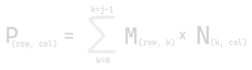
Consider a matrix M of shape i x j and a matrix N of shape j x k, such that multiplication of the matrix produces another matrix P, of shape i x k. Mathematically, it is given by:

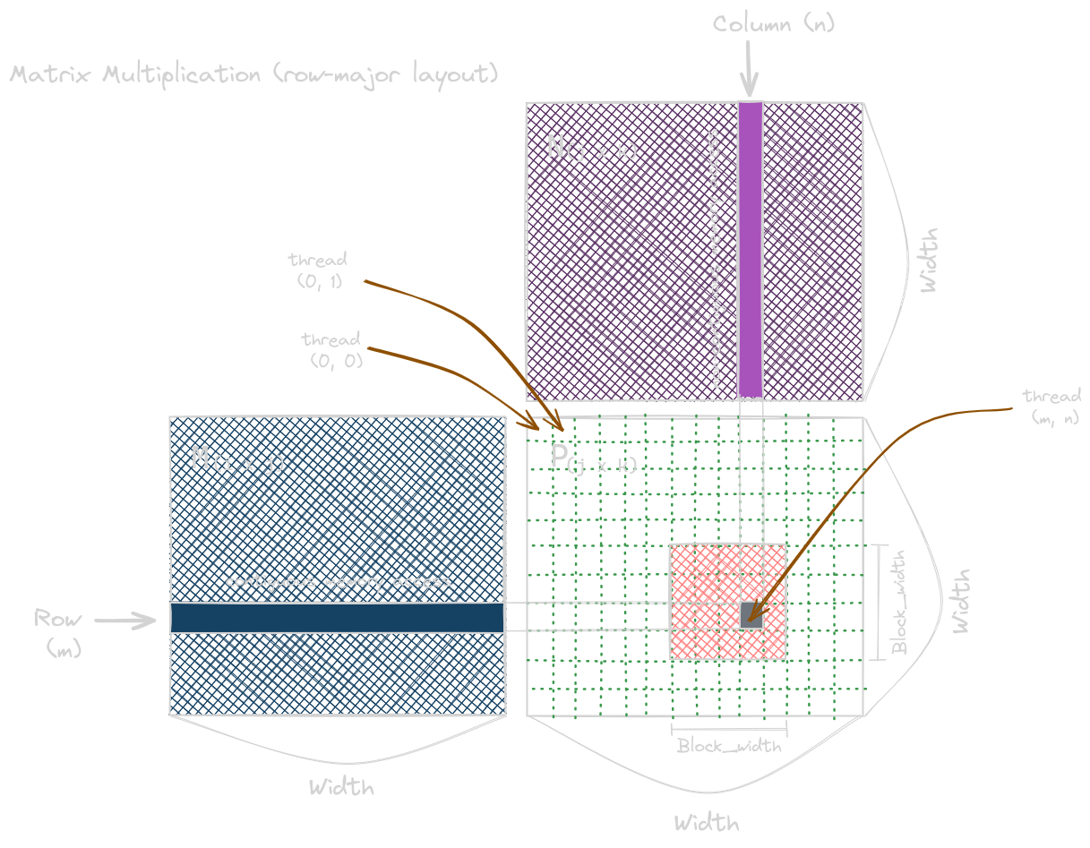
The matrix multiplication kernel below is the one-to-one mapping; the row and column thread indices are also the row and column indices for their output elements. Note that the kth element of the rowth row is at M[row * Width + k]. And the kth element of the colth col is at N[k * Width + col].

__global__ void matrixMulKernel(float* M, float* N, float* P, int width) {
    int col = threadIdx.x + blockIdx.x * blockDim.x;
    int row = threadIdx.y + blockIdx.y * blockDim.y;

    if ((row < width) && (col < width)) {
        float Pvalue = 0;
        for (int k = 0; k < width; k++) {
            Pvalue += M[row * width + k] * N[k * width + col];
        }
        P[row * width + col] = Pvalue;
    }
}

Let’s demonstrate the work done by each thread. We see each P_{(row, col)} is calculated as an inner product of the rowth row of M and colth col of N in the for-loop. For a matrix multiplication of two 4092² matrices followed by an addition of a 4092² matrix (for GEMM), the total FLOPS, total data read, and the actual data stored is given by:

• Total FLOPS: 2 * 4092³ + 4092² = 137 GFLOPS
• Total data to read (minimum!): 3 * 4092² * 4B = 201MB
• Total data to store: 4092² * 4B = 67MB

This example is taken from “How to Optimize a CUDA Matmul Kernel for cuBLAS-like Performance: a Worklog”².

Conclusion

That’s all for this blog. We started our journey by understanding the three-level thread hierarchy, the memory layout of the dynamically allocated arrays, and their rearrangement into 1D arrays while computing. We then demonstrated the mechanics of multi-dimensional array processing via various examples like color-to-gray-scale conversion, image blurring, and the naive implementation of matrix multiplication. In the upcoming series, we’ll learn about the basics of compute architecture and scheduling of the algorithms to optimize our naive matrix multiplication kernel implementation.

Where to Go Next?

I hope you enjoyed reading this blog post! If you have any questions or suggestions, please feel free to drop a comment or reach out to me. I’d love to hear from you!

This post is part of an ongoing series on CUDA programming. I plan to continue this series and keep things exciting. Check out the rest of my CUDA blog series:

1. Introduction to Parallel Programming and CPU-GPU Architectures
2. Multidimensional Grids and Data
3. Compute Architecture and Scheduling
4. Memory Architecture and Data Locality
5. Performance Considerations
6. Convolution
7. Stencil
8. Parallel Histogram
9. Reduction

Stay tuned for more!

Resources & References

1. Wen-mei W. Hwu, David B. Kirk, Izzat El Hajj, Programming Massively Parallel Processors: A Hands-on Approach, 4th edition, United States: Katey Birtcher; 2022
2. How to Optimize a CUDA Matmul Kernel for cuBLAS-like Performance: a Worklog; Dec 2022
3. Recap Ch. 1-3 from the PMPP book YouTube by Andreas Koepf; Dec 2024
4. Lecture 3: Getting Started With CUDA for Python Programmers by Jeremy Howard; Jan 2024
5. I used Excalidraw to draw the kernels.