Introduction to Parallel Programming and CPU-GPU Architectures
Hi there! I’ve been diving into the world of parallel programming from the excellent book “Programming Massively Parallel Processors: A Hands-on Approach1” by Wen-mei W. Hwu, David B. Kirk, and Izzat El Hajj. The content of this blog post is motivated by the book’s first chapter: Introduction, the second chapter: Heterogeneous data-parallel Computing, and the Intel blogs2 on vectorization.
I often see folks working on the speed of execution of programs in GPUs and CPUs and reach the conclusion GPUs outperform in many cases. Well, there’s a lot of interesting stuff under the hood.
Introduction
The evolution of microprocessors began in the early 1980s. Initially, there was rapid growth in performance on increasing the clock speed. However, after the 2003s, it took a lot of work for the companies to improve due to heating issues, so the companies came up with the idea to add more number of processor cores to increase their processing power. From a single-core processor to a double-core processor, then to a multicore processor (typically just increasing the number of physical CPUs, but the operations were performed in sequential steps). It brought significant changes, but the technique does not actually increases the speed of execution of the microprocessor; it just adds another processor core. We know performance is a never-ending process, and we need technology to produce realistic effects. NVIDIA introduced a new generation of microprocessors back in the 1990s, which could run software applications using multiple threads, The threads can cooperate with each other and run parallelly, leading to a significant increase in performance for a larger number of input data. Since then, there have been notable developments in processor speed. Let’s dig in more about parallel computing.
Heterogeneous parallel computing
Following up on the earlier introduction. We saw how the processor evolved by the time. And the two different designs were introduced, one by Intel & AMD (latency-oriented design) and the other by NVIDIA (throughput-oriented design).
- Multicore Trajectory: The team increased the number of processor/ CPU cores generation after generation to increase the performance. Since they have multiple cores, they can process multiple instructions simultaneously, but the new execution of the subsequent instructions starts after the completion of one instruction. The most recent Intel processor has a 24-core, which could run 0.33 TFLOPS for FP64i1 and 0.66 TFLOPS for FP321.
- Many Threaded Trajectory: In this trajectory, many cores will perform their operations parallelly, irrespective of the other cores. The support of the number of threads that can run in parallel was increased generation after generation. The most recent NVIDIA arch can run 9.7 TFLOPS for FP641, 156 TFLOPS for FP321, and 312 TFLOPS for FP161 datatypes, which are incredible results compared to multicore trajectories.
Why is there such a large peak performance difference between multicore CPU and many-thread GPU?
The answers lie within the core design structure the companies selected to follow: the CPUs are designed to optimize the sequential code, while the GPUs are designed to perform a massive number of operations simultaneously. Please see the pictures below, which depict the fundamental architectural difference between the CPU and the GPU.
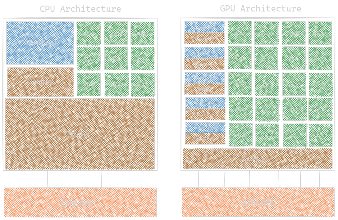
- The amount of space for an Arithmetic Logic Unit (ALU) in the CPU is comparatively very small compared to the GPU. The reason is we only need to perform sequential operations in CPU, so Intel dedicated a small amount of space for performing these operations, while in GPU, we need more space to accommodate as many operations as possible, so NVIDIA dedicated more space to it; the latest GPUs (Tesla P100, Tesla V100, A100) support 1024 threads per block (we’ll get into more details about this in later blog posts).
- On the other hand, more data needs to be stored in CPU memory because they will be waiting for their turn to execute, so Intel dedicated more space for Cache memory in their processors. In comparison, NVIDIA GPUs don’t really require more space to hold the data, so they dedicated less space for Cache memory. The NVIDIA GPUs show remarkable performance, but things are challenging because the speed depends on how data can be delivered from the host memory to global memory, then to the shared memory & registers inside the processor block, and vice versa. We will read more about this topic in my upcoming blog posts.
- Coming back to the point, Intel’s goal is to reduce the latency of an operation so that many operations can be completed in a short time interval, while NVIDIA’s goal is to increase the number of operations performed at a single instant, aka throughput oriented.
Over time, it was observed that GPUs perform great when we have to perform many operations simultaneously. But still, under the hood, GPUs cannot completely replace the use of CPUs; we need to use host memory for a smaller number of operations.
This led to the introduction of CUDA (Compute Unified Device Architecture). NVIDIA designed it to support the joint execution of CPU-GPU applications and for General Purpose Parallel Programming (GPGPU). GPGPUs are used to perform general mathematical computations on GPUs. NVIDIA added additional hardware to the chip to run these programs. And the speed of execution depends on the amount of data that can be parallelized. But keep in note the most crucial factor in speeding up is how fast you can read and write the data from memory. Various fusion methods and parallelization techniques are developed to decrease the gaps between the hardware and software integration which we’ll read later. Let’s hop into some important considerations we need to have if we want to write a CUDA program:
- identify the part of application programs to be parallelized
- isolating the data to be used by the parallelized code
- using an API function to transfer data to the parallel computing device
- developing parallel part into a kernel function for execution by parallel threads
- launching a kernel function for the execution of parallel threads
- eventually, transferring the data back to the host processor with an API function call
Let’s try some CUDA and Vectorized Code Examples
Here’s an example of vector addition in NVIDIA GPUs using CUDA. We created a
function in host memory (vecAdd) that asynchronously launches vecAddKernel
initiated in the global memory (memory that can be written and read from both
host and device, basically, it’s an entry point to every device code).
Kernel functions specify all threads should execute on different parts of data.
It shows a single program is splitting across multiple data in GPUs, aka SPMD.
If you are curious and searching about how to call __host__, __device__, and __global__
functions, check out my Stack Overflow answer.
#include <iostream>

// access by both __host__ & __device__ functions
__global__ void vecAddKernel(float* A, float* B, float* C, int n) {
    // local variable `i` & n, generated for each thread in a register
    // each thread follows the SIMD process
    // threadIdx.x: index of current thread inside a block
    // blockDim.x: number of threads in a block
    // blockIdx.x: index of block inside a grid
    // gridDim.x: number of blocks in a grid
    int i = threadIdx.x + blockDim.x * blockIdx.x;
    if (i < n) {  // memory bound check
        C[i] = A[i] + B[i];
    }
}

// host memory
void vecAdd(float* A_h, float* B_h, float* C_h, int n) {
    // size in bytes
    int size = n * sizeof(float);
    float *A_d, *B_d, *C_d;

    cudaEvent_t start, stop;
    cudaEventCreate(&start);
    cudaEventCreate(&stop);

    // allocating memory in GPU, the function accepts a generic pointer
    // returns generic objects
    // adding error checks
    cudaError_t allocErr;
    allocErr = cudaMalloc((void**)&A_d, size);
    if (allocErr != cudaSuccess) {
        std::cerr << "A_d: " << cudaGetErrorString(allocErr) << std::endl;
        return;
    }
    allocErr = cudaMalloc((void**)&B_d, size);
    if (allocErr != cudaSuccess) {
        std::cerr << "B_d: " << cudaGetErrorString(allocErr) << std::endl;
        cudaFree(A_d);
        return;
    }
    allocErr = cudaMalloc((void**)&C_d, size);
    if (allocErr != cudaSuccess) {
        std::cerr << "C_d: " << cudaGetErrorString(allocErr) << std::endl;
        cudaFree(A_d);
        cudaFree(B_d);
        return;
    }

    // to transfer (synchronous) data from host to device
    cudaMemcpy(A_d, A_h, size, cudaMemcpyHostToDevice);
    cudaMemcpy(B_d, B_h, size, cudaMemcpyHostToDevice);

    dim3 dimGrid((n + 255) / 256, 1, 1);  // number of threads in each block
    dim3 dimBlock(256, 1, 1);  // number of blocks in a grid

    cudaEventRecord(start);
    vecAddKernel<<<dimGrid, dimBlock>>>(A_d, B_d, C_d, n);
    cudaEventRecord(stop);

    cudaMemcpy(A_h, A_d, size, cudaMemcpyDeviceToHost);
    cudaMemcpy(B_h, B_d, size, cudaMemcpyDeviceToHost);
    cudaMemcpy(C_h, C_d, size, cudaMemcpyDeviceToHost);

    // to free storage space of global memory
    cudaFree(A_d);
    cudaFree(B_d);
    cudaFree(C_d);

    cudaEventSynchronize(stop);
    float milliseconds = 0;
    cudaEventElapsedTime(&milliseconds, start, stop);
    std::cout << milliseconds << std::endl;
}

int main() {
    int n = 1000000;
    // dynamically allocate arrays
    // (for larger numbers, normal allocation leads to memory issues)
    float *A_h = new float[n];
    float *B_h = new float[n];
    float *C_h = new float[n];

    for(int i = 0; i < n; i++) {
        A_h[i] = static_cast<float>(i + 1);
        B_h[i] = static_cast<float>(n - i - 1);
    }

    vecAdd(A_h, B_h, C_h, n);

    delete[] A_h;
    delete[] B_h;
    delete[] C_h;

    return 0;
}
Let’s see a vector addition example in Intel CPUs using vectorization.
Vectorization is a way to write parallel operations in CPUs.
In modern CPUs, these are implemented via Advanced Vector Extensions (AVX);
some of their types are AVX1, AVX2, AVX512, etc. We’ll use AVX128 in our example.
In CPUs, each instruction processes multiple data, aka SIMD.
Note that each intrinsic operation is placed in a
register—for more info, check on
Intel’s blog on Intrinsics2.
In the code below, _mm_loadu_ps(), _mm_add_ps, and _mm_store_ps
are built-in variables for loading the packed single-precision data
from a memory to aligned memory, adding two single precision data
and storing the packed single precision floating point values from a
float32 vector to an aligned memory location.
The compiler can generate optimized results directly from the intrinsic vector.
PS: This information is just a few things I learned by stumbling on the
internet/Intel blogs.
#include <benchmark/benchmark.h>
#include <emmintrin.h>  // to include Intel's SSE2 intrinsics
#include <iostream>

void vecAdd(float* A, float* B, float* C, int n) {
    for (int i = 0; i < n; i += 4) {
        // _m128: it is a data type with SIMD extensions
        // defined on 16-byte boundaries, similar to int, long dtypes
        // it reverses the order of the arguments by convention
        __m128 v1 = _mm_loadu_ps(&A[i]);
        __m128 v2 = _mm_loadu_ps(&B[i]);

        __m128 r = _mm_add_ps(v1, v2);

        _mm_store_ps(&C[i], r);
    }
}

static void BM_vecAdd(benchmark::State& state) {
    const int n = state.range(0);
    float *A = new float[n];
    float *B = new float[n];
    float *C = new float[n];

    for(int i = 0; i < n; i++) {
        A[i] = static_cast<float>(i + 1);
        B[i] = static_cast<float>(n - i - 1);
    }

    for (auto _ : state) {
        vecAdd(A, B, C, n);
    }

    delete[] A;
    delete[] B;
    delete[] C;
}

BENCHMARK(BM_vecAdd)->Arg(1000000);
BENCHMARK_MAIN();
Performance Benchmarking
Let’s benchmark our code and verify the results with the theoretical explanations above. Before hopping in, all the performance results below are taken from NVIDIA GEFORCE GTX 1650Ti and Intel(R) Core(TM) i7-10870H.
I used Google Benchmark4 to benchmark the CPU’s
vecAdd function above and CUDA Events3
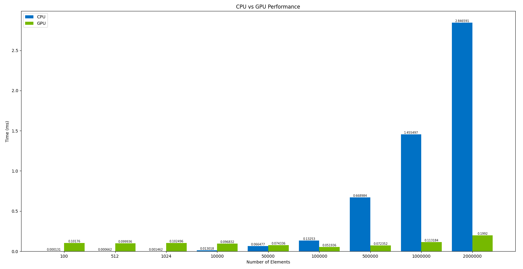
to benchmark the CUDA kernel vecAddKernel above. We found
remarkable results, initially for 100 input values; the results shown by
CPU were 776.79 times faster than NVIDIA GPUs. OMG! That’s way too huge.
But the exciting thing about increasing the number of particles: NVIDIA
GPUs showcased exceptional speed and performance while the Intel processor got way
too much slower. For 2M input values, GPUs outperform the CPUs by 14.2
times. And this gap will increase with the increase in the number of
input values. So, you should use CPUs for a smaller number of inputs
but rely on GPUs for larger input values.
That said, things are about more than just replacing one another;
it’s about utilizing the most adequate thing per the user’s requirement.
| n | tCPU(ms) | tGPU(ms) |
|---|---|---|
| 100 | 0.000131 | 0.10176 |
| 512 | 0.000662 | 0.099936 |
| 1024 | 0.001462 | 0.102496 |
| 10000 | 0.013018 | 0.096832 |
| 50000 | 0.066477 | 0.074336 |
| 100000 | 0.13253 | 0.051936 |
| 500000 | 0.668984 | 0.072352 |
| 1000000 | 1.455497 | 0.113184 |
| 2000000 | 2.846591 | 0.1992 |
Please view the graphical representation of the same:
Conclusion
So, had fun? This blog post was just a gentle introduction to parallel programming. We started the blog posts with the evolution of CPUs, which led to the introduction of GPUs. We then read about how their architectural designs cause such a huge difference in performance. Later, we ended the blog posts by playing with some cool examples to write a vector addition kernel in CUDA and CPU via vectorization and benchmarked them.
I hope you enjoyed it! I would love to know your thoughts and anything interesting you’ve learned in your journey to understanding parallel programming. Feel free to leave a comment below. See you next time in my upcoming exciting blog post for writing an optimized Matrix Multiplication kernel! Stay tuned!
Acknowledgement
Thanks to Kshitij Kalambarkar for reading the initial drafts of the blog posts and providing feedback & suggestions on them.
Where to Go Next?
I hope you enjoyed reading this blog post! If you have any questions or suggestions, please feel free to drop a comment or reach out to me. I’d love to hear from you!
This post is part of an ongoing series on CUDA programming. I plan to continue this series and keep things exciting. Check out the rest of my CUDA blog series:
- Introduction to Parallel Programming and CPU-GPU Architectures
- Multidimensional Grids and Data
- Compute Architecture and Scheduling
- Memory Architecture and Data Locality
- Performance Considerations
- Convolution
- Stencil
- Parallel Histogram
- Reduction
Stay tuned for more!
Resources & References
1. Wen-mei W. Hwu, David B. Kirk, Izzat El Hajj, Programming Massively Parallel Processors: A Hands-on Approach, 4th edition, United States: Katey Birtcher; 2022
2. Intel developers, Intel Intrinsics Guide, Updated on May 10, 2023
3. Mark Harris, Implement Performance Metrics, NVIDIA Technical Blog, November 07, 2012
4. Google’s microbenchmark support library, benchmark
5. I used Excalidraw to draw the kernels.
Let me know what you think of this article on Twitter @khushi__411 or leave a comment below!