Memory Architecture and Data Locality
Introduction
Hi there! The blog posts aim to study the GPUs’ on-chip memory architecture and how to organize and position data for efficient thread access. Until now, we executed our programs all from global memory access (off-chip DRAM), which leads to delays and traffic and negatively affects performance. In this blog post, we will study ways to tolerate these long-latency operations, i.e. we’ll introduce various techniques to reduce global memory access.
This blog post is written while reading the fifth chapter, Memory Architecture and Data Locality of the amazing book “Programming Massively Parallel Processors: A Hands-on Approach1” by Wen-mei W. Hwu, David B. Kirk, and Izzat El Hajj.
Importance of memory access Efficiency
For matrix multiplication, in every iteration in a for-loop, two global memory accesses are performed, one for floating-point multiplication and the other for its addition. This ratio of floating-point operations (FLOPS) to bytes (B) accessed from the global memory is called arithmetic intensity or computational intensity. The execution of the matrix multiplication kernel is limited by the rate at which data can be delivered from the memory to the GPU cores. Such executions are referred to as memory-bound programs.
For example, the Ampere GPUs have a peek memory bandwidth of 1555 GB/sec, and the number of GFLOPS performed is 19,500. Therefore, the computational intensity will be 19,500 / 1555 = 12.5 Operations per byte. That means that to fully utilize every 4 bytes of memory, 50 operations must be performed.
Hence, the programmer must determine the relative case of the program’s compute-bound and memory-bound scenarios to write a performant model.
CUDA Memory Types
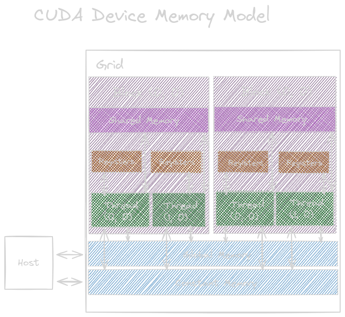
From the figure above, here is a short description of the CUDA memory types:
- Global Memory: It is read and written by the hosts and the device. It is off the processor chip. It has long-latency operations, hence slower.
- Constant Memory: It is read and written by
the hosts but only read by the device
(short latency and high bandwidth).
- Constant variables are placed in global memory but cached into constant memory for efficient access.
- Local Memory: It is placed in the global memory; it can be read and written but not shared across the threads. Each thread has its own section of private local memory that cannot be shared or allocated to the registers.
- Shared Memory: This is on-chip memory with high-speed access. It is allocated to thread blocks, so access to all the threads is across the blocks; that’s how threads interact with each other. It resides on a processor chip. Lower latency and higher throughput than global memory but higher than registers. Variables that reside inside this are visible to all threads within that block.
- Registers: These are on-chip memory with
high-speed access and are allocated to individual
threads. Kernel functions use these registers
to hold private variables and data. They are on the
processor chip, therefore, high-speed and short-latency
operations. Processing an instruction involves a few instructions.
- When an operand is already on the register, no additional instructions are involved to make the operand available for the arithmetic and logic unit (ALU).
CPUs save the registers from going to memory by switching between different threads, while GPUs achieve zero-overhead scheduling by keeping the registers scheduled during the process.
When an operand is in the global memory, the instruction stack:
load r2, r4, offset;
fadd r1, r2, r3;
When an operand is in the register, the instruction stack (hence improves the performance):
fadd r1, r2, r3;
The scope of the CUDA variable is determined by the number of threads that can access the variables, i.e., single thread only, all threads in a block, or all threads of all grids.
| Variable Declaration | Memory | Scope | Lifetime |
|---|---|---|---|
| Automatic variables other than arrays | Register | Thread | Grid |
| Automatic array variables | Local | Thread | Grid |
| __device__ __shared__ int SharedVar; | Shared | Block | Grid |
| __device__ int GlobalVar; | Global | Grid | Application |
| __device__ __constant__ int ConstVar; | Constant | Grid | Application |
Tiling for reduced memory traffic
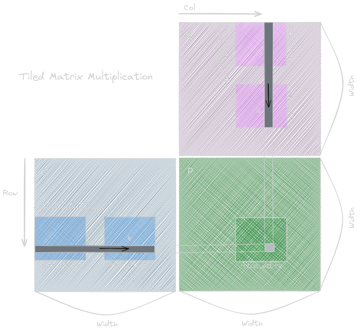
To store less data for faster computation, we will store it in shared memory. We will partition the data into smaller portions known as tiles and then store them. For example, in the matrix multiplication shown in my previous blog of this series. There will be multiple threads accessing the same data from the global memory multiple times; this will make the process slower. We need to find a way to collaborate with these threads so that they can access these data from global memory only once. This will lead to a potential reduction in global memory traffic.
This led to the introduction of the Tiled Matrix Multiplication algorithm. The algorithm states that we first load the subsets of matrix M and N (by dividing them into tiles) into the shared memory before performing any calculations, then calculate the products and additions.
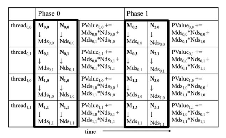
The above image from the book shows the activities of threads in block(0,0). The shared memory elements for arrays M and N are called Mds and Nds. These Mds and Nds remain in the shared memory and are reused across multiple phases. Hence, it saves us from relying on global memory to access data from them. Each phase focuses on a small subset of data from the input matrix multiplication, known as locality.
Tiled Matrix Multiplication Kernel
As shown below:
__global__ void matrixMulKernel(float* M, float* N, float* P, int Width) {

    // shared memory arrays
    __shared__ float Mds[TILE_WIDTH][TILE_WIDTH];
    __shared__ float Nds[TILE_WIDTH][TILE_WIDTH];

    // automatic variables
    int bx = blockIdx.x;
    int by = blockIdx.y;
    int tx = threadIdx.x;
    int ty = threadIdx.y;

    // calculate the row and column of the P element
    int row = by * TILE_WIDTH + ty;
    int col = bx * TILE_WIDTH + tx;

    float Pvalue = 0;
    for (int ph = 0; ph < Width/TILE_WIDTH; ++ph) {

        // collaborative loading of M and N tiles into the shared memory
        Mds[ty][tx] = M[row*Width + ph*TILE_WIDTH + tx];
        Nds[ty][tx] = N[(ph*TILE_WIDTH + ty) * Width + col];

        // read-after-write data dependence
        __syncthreads();

        for (int k = 0; k < TILE_WIDTH; ++k) {
            Pvalue += Mds[ty][k] * Nds[k][tx];
        }

        // write-after-read data dependence
        __syncthreads();
    }
    P[row*Width + col] = Pvalue;
}
Mathematically, we reduce the global memory access ratio by the factor of TILE_WIDTH. For example, if we have a matrix of size 16 x 16, by using a tiled matrix multiplication algorithm, we’ll reduce the access by a factor of 16. This increases the compute-to-global memory access ratio from 0.25 OP/B (via naive impl, as calculated earlier) to 4 OP/B.
Boundary Checks
To handle matrices whose width is not a multiple of tile width.
    float Pvalue = 0;
    for (int ph = 0; ph < ceil(Width/(float)TILE_WIDTH); ++ph) {

        // collaborative loading of M and N tiles into the shared memory
        if ((row < Width) && (ph*TILE_WIDTH + tx) < Width) {
            Mds[ty][tx] = M[row*Width + ph*TILE_WIDTH + tx];
        } else {
            Mds[ty][tx] = 0.0f;
        }

        if ((ph*TILE_WIDTH + ty) < Width && col < Width) {
            Nds[ty][tx] = N[(ph*TILE_WIDTH + ty) * Width + col];
        } else {
            Nds[ty][tx] = 0.0f;
        }

        // read-after-write data dependence
        __syncthreads();

        for (int k = 0; k < TILE_WIDTH; ++k) {
            Pvalue += Mds[ty][k] * Nds[k][tx];
        }

        // write-after-read data dependence
        __syncthreads();
    }

    if ((row < Width) && (col < Width)) {
        P[row*Width + col] = Pvalue;
    }
Where to Go Next?
I hope you enjoyed reading this blog post! If you have any questions or suggestions, please feel free to drop a comment or reach out to me. I’d love to hear from you!
This post is part of an ongoing series on CUDA programming. I plan to continue this series and keep things exciting. Check out the rest of my CUDA blog series:
- Introduction to Parallel Programming and CPU-GPU Architectures
- Multidimensional Grids and Data
- Compute Architecture and Scheduling
- Memory Architecture and Data Locality
- Performance Considerations
- Convolution
- Stencil
- Parallel Histogram
- Reduction
Stay tuned for more!
Resources & References
1. Wen-mei W. Hwu, David B. Kirk, Izzat El Hajj, Programming Massively Parallel Processors: A Hands-on Approach, 4th edition, United States: Katey Birtcher; 2022
2. Lecture 8: CUDA Performance Checklist; by Mark Saroufin; March 2024
3. I used Excalidraw to draw the kernels.
Let me know what you think of this article on Twitter @khushi__411 or leave a comment below!