Convolution

Introduction

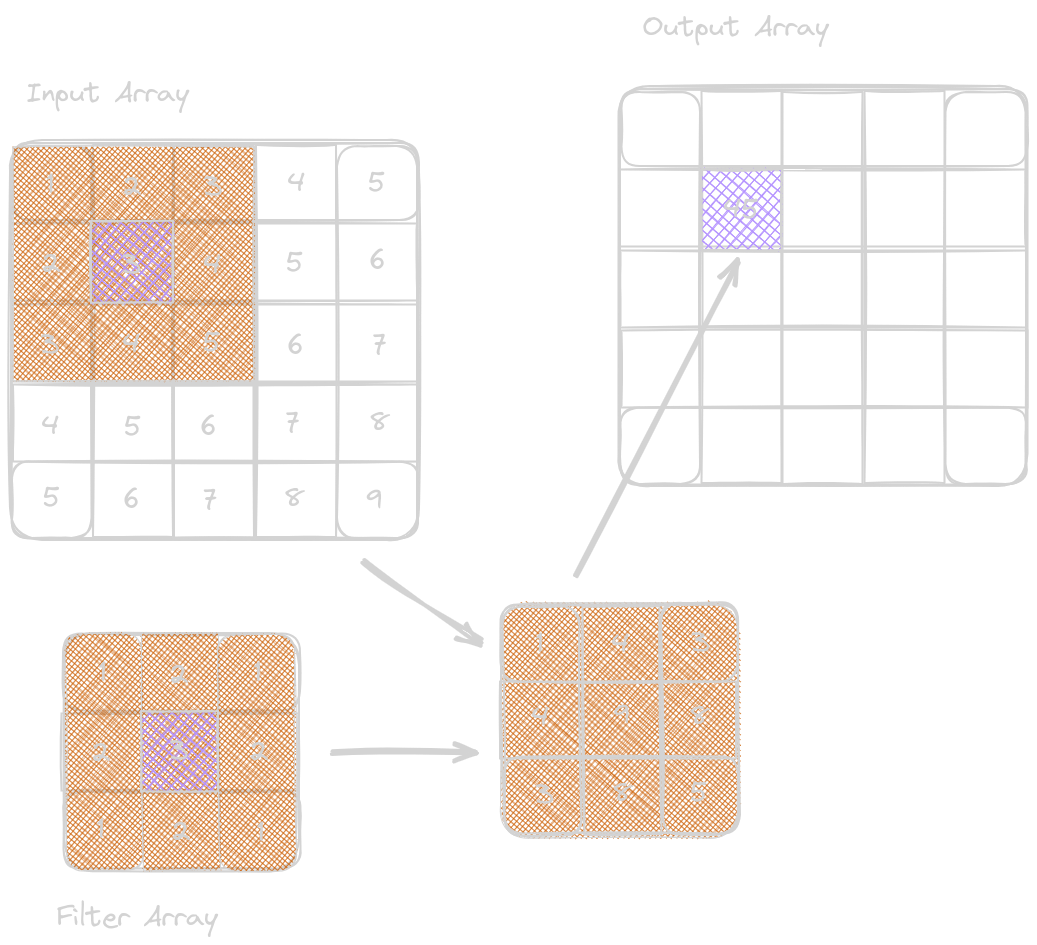
Convolution is an array operation used in various forms in signal processing, digital recording, image/video processing, and computer vision. In convolution, each output element is calculated independently as a weighted sum of the corresponding and surrounding input elements. These weights used in calculating the weighted sum are known as a filter array and are defined as a convolution kernel. However, processing large datasets efficiently poses significant challenges, so it becomes a sophisticated use case for advanced optimization techniques, such as tiling methods and input data staging methods.

In this post, we will explore the basics of convolution and dive into several optimization techniques. We’ll cover topics like constant memory and caching, tiled convolution with halo cells, and leveraging caches for halo cells to improve performance.

This blog post is written while reading the seventh chapter, Convolution, of the incredible book “Programming Massively Parallel Processors: A Hands-on Approach¹” by Wen-mei W. Hwu, David B. Kirk, and Izzat El Hajj.

Background

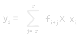
A convolution on 1D array is known as 1D convolution. Let n be the number of elements in the input array [x₀, x₁,…,x_n-1] and let 2r+1 elements in the filter array [f₀, f₁,…,f_2r] such that it returns an output array y. The size of the filter is an odd number, so it is symmetric around the element to be calculated.

A convolution on 2D arrays is known as 2D convolution. Let N be the 2-dimensional array, and f be the filter of dimension (2r_x+1) in the x-direction and (2r_y+1) in the y-direction. To output convoluted kernel is given by:

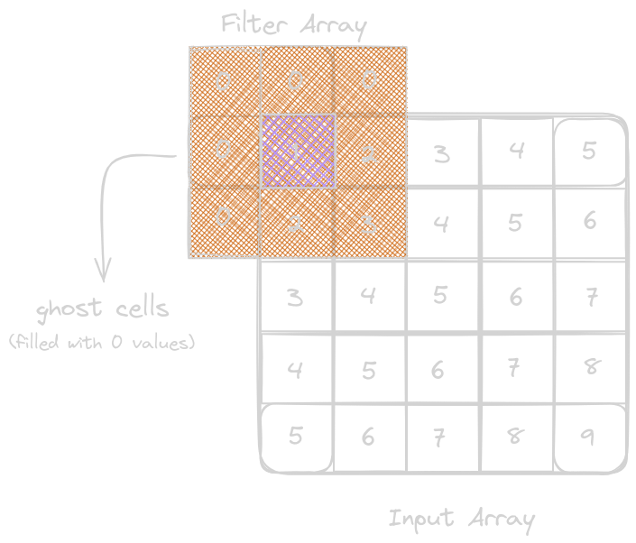
For the elements in the input array that do not exist for the calculation with the filter arrays, we create an imaginary element, either 0 or any other values; these cells with missing elements are known as ghost cells. These boundary conditions affect the efficiency of the tiling.

Parallel Convolution: a basic algorithm

__global__ void convolution_2d_basic_kernel(float* N, float* F, float* P,
    int r, int width, int height) {
    
    // To calculate the output element indices
    int outCol = blockIdx.x*blockDim.x + threadIdx.x;
    int outRow = blockIdx.y*blockDim.y + threadIdx.y;

    // Register variable
    float Pvalue = 0.0f;
    for (int fRow = 0; fRow < 2*r+1; fRow++) {
        for (int fCol = 0; fCol < 2*r+1; fCol++) {
            inRow = outRow - r + fRow;
            inCol = outCol - r + fCol;

            // There will be control flow divergence
            // It'll depend on the width and height of the
            // input array and radius of the filter
            // To handle ghost cells
            if (inRow >= 0 && inRow < height && inCol >= 0 && inCol < width) {
                Pvalue += F[fRow][fCol]*N[inRow*width + inCol];
            }   
        }   
    }   
    // Release Pvalue to the output element
    P[outRow][outCol] = Pvalue;
}

Constant Memory and Caching

Characteristics for an array to be implemented in the constant memory:

• The constant memory size is very small, ~ 64 KB. In order for an array to reside here, its size should be small. The filter array discussed above holds up a very small size (7 or less).
• The values of the variables should not change while executing in the kernel. For example, the filter values in the convolution kernel above do not change during execution.
• All threads should execute the elements of the filter array.

To declare any variable or array in constant memory, apply __constant__ to tell the compiler. The only difference is that while writing this kernel, we’ll not pass the filter array through a pointer as passed above; instead, the filter array will be accessed as a global variable.

Since constant memory variables are not modified during kernel execution, we don’t need to support writes into threads when caching them to the SM. Hence, this saves us from memory and power consumption. The variables/arrays stored in a form of cache here are highly effective and are known as constant cache. The constant cache provides a huge bandwidth to satisfy the data needs of these threads. This implies that no DRAM bandwidth is spent on accesses to the filter elements. It also implies that access to input elements also benefits from caching.

Tiled Convolution with Halo cells

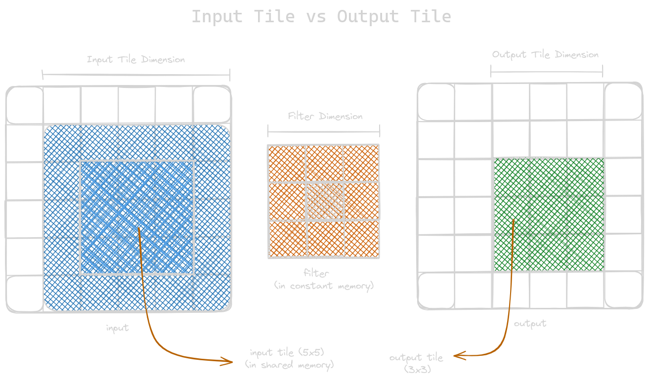
In the tiled convolution algorithm, all the threads in the block load the input tile to the shared memory and then load the registers to perform the desired operations. This section is similar to tiled matrix multiplication discussed in the previous blog; the only difference is that the dimensions of the input matrix are bigger than the dimensions of the resulting output matrix. We could address this difference in a number of input and output element dimensions in two ways.

• Launch thread blocks whose dimensions are equal to the input tiles. This simplifies loading the input tiles, but it becomes complex to map output elements because their size is smaller than the input tiles. So, we need to disable some threads while calculating the output element, which leads to reduced efficiency (we’ll follow this in our example below).
• Another approach is when the dimensions of the block is the same as that of the output element. But in this case, loading the input tile is complex to handle. In this case, we do not need to disable threads mapping output elements.

#define IN_TILE_DIM 32
#define OUT_TILE_DIM ((IN_TILE_DIM) - 2*(FILTER_RADIUS))

__constant__ float F_c[2*FILTER_RADIUS+1][2*FILTER_RADIUS+1];

__global__ void convolution_tiled_2D_const_mem_kernel(float *N, float *P,
    int width, int height) {

    // Each thread calculates the column and row index of the input
    int col = blockIdx.x*OUT_TILE_DIM + threadIdx.x - FILTER_RADIUS;
    int row = blockIdx.y*OUT_TILE_DIM + threadIdx.y - FILTER_RADIUS;

    // Loading input tile into the shared memory
    __shared__ N_s[IN_TILE_DIM][IN_TILE_DIM];

    // To check whether the input tile is a ghost cell or not
    if (row >= 0 && row < height && col >= 0 && col < width) {
        N_s[threadIdx.y][threadIdx.x] = N[row*width + col];
    } else {
        N_s[threadIdx.y][threadIdx.x] = 0.0;
    }
    __syncthreads();

    // Calculating output elements
    // We'll deactivate FILTER_RADIUS = 1 exterior layer of threads
    // Mapping active threads to the output tile elements
    int tileCol = threadIdx.x - FILTER_RADIUS;
    int tileRow = threadIdx.y - FILTER_RADIUS;

    // Turning off the threads at the edges of the block
    if (col >= 0 && col < width && row >= 0 && row < height) {
        if (tileCol >= 0 && tileCol < OUT_TILE_DIM && tileRow >= 0 && tileRow < OUT_TILE_DIM) {
            float Pvalue = 0.0f;
            for (int fRow = 0; fRow < 2*FILTER_RADIUS+1; fRow++) {
                for (int fCol = 0; fCol < 2*FILTER_RADIUS+1; fCol++) {
                    Pvalue += F[fRow][fCol]*N_s[tileRow+fRow][tileCol+fCol];
                }
            }
            P[row*width+col] = Pvalue;
        }
    }
}

Tiled Convolution using Caches for halo cells

Tiled convolution algorithm that uses the same dimensions for input and output tiles and loads only internal elements of each tile into the shared memory. Note that the halo cells of an input tile of a block are also internal elements of neighbouring tiles. There is a possibility that while computing the values, the element at halo cells resides on L2 cache memory, hence saving us from the DRAM traffic. We can leave the halo cells in the original tiles rather than loading them to the shared memory.

#define TILE_DIM 32

__constant__ float F_c[2*FILTER_RADIUS+1][2*FILTER_RADIUS+1];

__global__ void convolution_cached_tiled_2D_const_mem_kernel(float *N,
    float *P, int width, int height) {

    // Simplified version of the earlier kernel
    // because now we are not loading halo cells
    // into the shared memory
    int col = blockIdx.x*TILE_DIM + threadIdx.x;
    int row = blockIdx.y*TILE_DIM + threadIdx.y;

    // Loading input tile
    __shared__ N_s[TILE_DIM][TILE_DIM];

    // Simplified version of the earlier kernel
    // because now we are not loading halo cells
    // into the shared memory
    if(row < height && col < width) {
        N_s[threadIdx.y][threadIdx.x] = N[row*width + col];
    } else {
        N_s[threadIdx.y][threadIdx.x] = 0.0;
    }
    __syncthreads();

    // Calculating output elements
    // Turning off the threads at the edges of the block
    if (col < width && row < height) {
        float Pvalue = 0.0f;
        for (int fRow = 0; fRow < 2*FILTER_RADIUS+1; fRow++) {
            for (int fCol = 0; fCol < 2*FILTER_RADIUS+1; fCol++) {
                // Handling of halo cells
                if (threadIdx.x-FILTER_RADIUS+fCol >= 0 &&
                    threadIdx.x-FILTER_RADIUS+fCol < TILE_DIM &&
                    threadIdx.y-FILTER_RADIUS+fRow >= 0 &&
                    threadIdx.y-FILTER_RADIUS+fRow < TILE_DIM) {
                  Pvalue += F[fRow][fCol]*N_s[threadIdx.y+fRow][threadIdx.x+fCol];
               } else {
                   // Check if the halo cells are ghost cells or not
                   if (row-FILTER_RADIUS+fRow >= 0 &&
                       row-FILTER_RADIUS+fRow < height &&
                       col-FILTER_RADIUS+fCol >=0 &&
                       col-FILTER_RADIUS+fCol < width) {
                     Pvalue += F[fRow][fCol]*N[(row-FILTER_RADIUS+fRow)*width
                       +col-FILTER_RADIUS+fCol];
                  }
              }
           }
           P[row*width+col] = Pvalue;
       }
    }
}

Where to Go Next?

I hope you enjoyed reading this blog post! If you have any questions or suggestions, please feel free to drop a comment or reach out to me. I’d love to hear from you!

This post is part of an ongoing series on CUDA programming. I plan to continue this series and keep things exciting. Check out the rest of my CUDA blog series:

1. Introduction to Parallel Programming and CPU-GPU Architectures
2. Multidimensional Grids and Data
3. Compute Architecture and Scheduling
4. Memory Architecture and Data Locality
5. Performance Considerations
6. Convolution
7. Stencil
8. Parallel Histogram
9. Reduction

Stay tuned for more!

Resources & References

1. Wen-mei W. Hwu, David B. Kirk, Izzat El Hajj, Programming Massively Parallel Processors: A Hands-on Approach, 4th edition, United States: Katey Birtcher; 2022
2. I used Excalidraw to draw the kernels.